Rain in the Driest Desert on Earth
Why northern Chile is flooding in 2026, and what El Niño has to do with it
Northern Chile sits close to home for me. My family lives there now, even though I was born in the V region myself, so this is not a story I am watching from a comfortable distance.
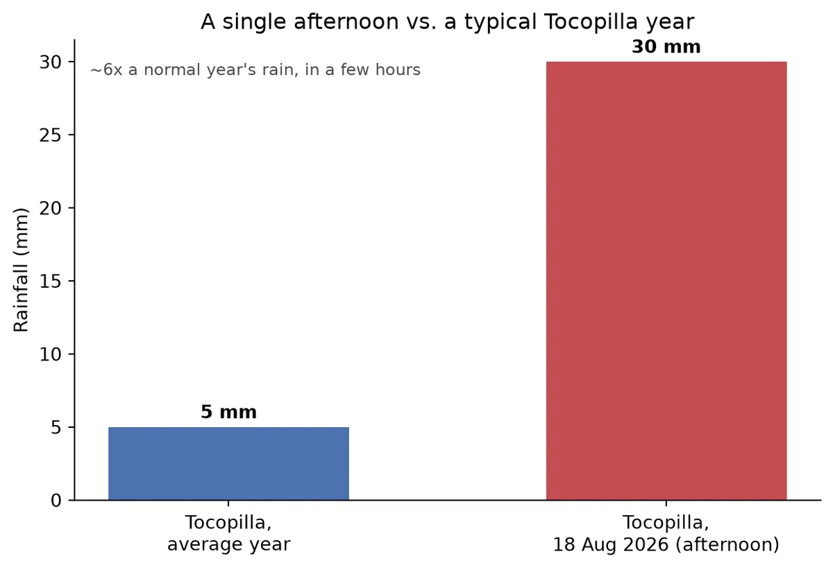
On the afternoon of 18 August 2026, about 30 millimetres of rain fell on Tocopilla, a port town of roughly 25 000 people in Chile’s Antofagasta region (II region). Tocopilla’s long term average is close to 5 millimetres a year. A cutoff low, a pocket of cold air that had pinched itself off from the main westerly flow over the Pacific, drew in enough moisture to dump something like six ordinary years of rain onto a town whose hillsides, drainage channels, and storm drains are built for a place that essentially never sees a storm at all [2]. The result was a mudflow through the streets, vehicles swept off roads, three neighbourhoods evacuated, one person killed by falling rock, three more missing, and a presidential declaration of a state of catastrophe for Tocopilla province [1] [2].
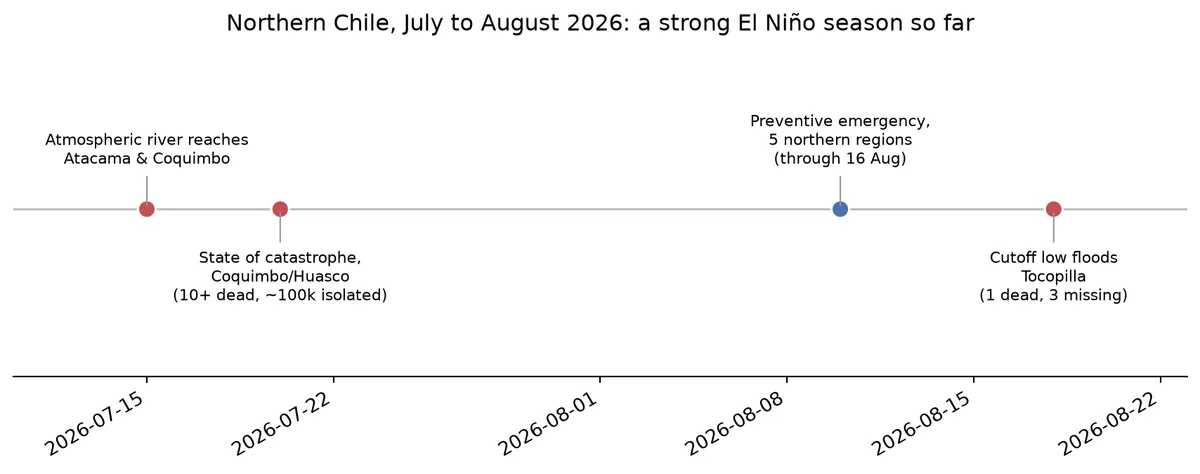
That was not an isolated event. It came eight days after Chile’s interior ministry had already declared a preventive weather emergency across five northern regions, Arica y Parinacota, Tarapacá, Antofagasta, Atacama, and Coquimbo, running from 10 to 16 August, in anticipation of exactly this kind of system [4]. And it came a month after a much larger storm, beginning around 15 July, killed at least ten people, left roughly 100 000 residents cut off by flooding, and forced a state of catastrophe in Coquimbo and Huasco [3] [5]. Some tallies of that July event later climbed into the double digits with several people still missing weeks on [6].
Three serious flood events in five weeks, in the part of the country least built to handle any rain at all, is worth asking a question about. What is actually driving this, and how much of it traces back to El Niño?
Where this actually happened
Antofagasta and Atacama are unfamiliar geography to a lot of readers, so it is worth placing Tocopilla on the map before going further. The preventive emergency covered five regions strung along roughly 1600 kms of coast, a sliver of land pinned between the Pacific and the Andes that rarely runs more than 150 kilometres wide, drawn below.
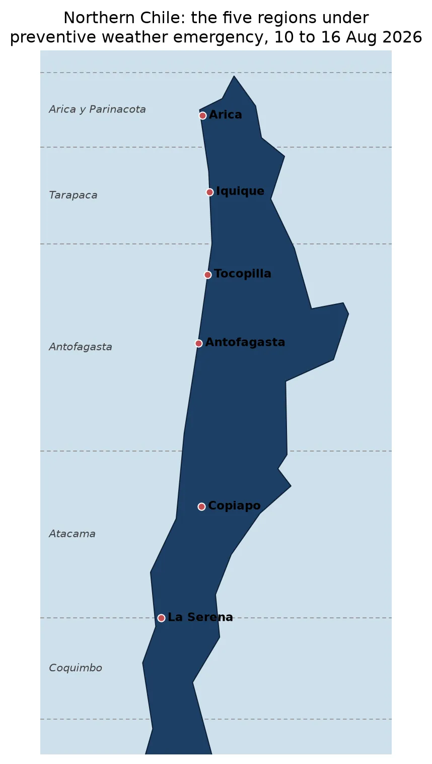
Tocopilla and Antofagasta sit almost on top of each other on this scale, about 190 km apart along the same short stretch of Antofagasta region coastline, which is part of why one cutoff low was able to leave a mark on both.
Why this desert is dry in the first place
It helps to start with why the Atacama is the driest non polar place on Earth in an ordinary year, because the flood driver has to work against three separate mechanisms that usually keep it bone dry.
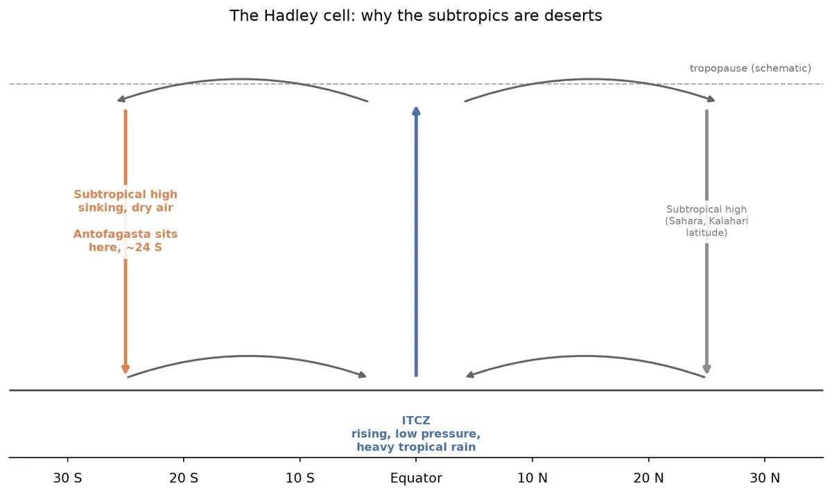
The first is circulation. Antofagasta sits under the sinking branch of the Hadley cell, the large scale overturning of tropical air that rises near the equator and descends again around 20 to 30 degrees south. Descending air warms and dries as it falls, which suppresses the cloud formation that rain depends on almost everywhere on the planet at this latitude, not just in Chile: the Sahara, the Kalahari, and central Australia sit under the same descending branch in their own hemisphere.
The second is the Humboldt Current, the cold water that runs north along Chile’s coast from the Southern Ocean. Cold water chills and stabilises the air sitting just above it, which locks a shallow layer of cool, stable air against the coast and keeps whatever moisture is there from rising far enough to condense into rain.
The third is the Andes. Moist air arriving from the Amazon basin on easterly winds is forced up and over the mountains, cools, and rains out on the eastern slopes long before it can reach the Pacific side. Antofagasta sits in the rain shadow of that process.
Three independent reasons for dryness stacked on top of each other is why the Atacama can go decades between one meaningful rain event and the next in its driest patches, and why a single afternoon of rain there makes international news in a way that the same rainfall would not anywhere else in Chile.
What actually broke through
Both August events reported so far this year had a specific proximate cause, and the two causes were not quite the same kind of system.
The July storm was described by meteorologists as an atmospheric river, a long narrow filament of concentrated water vapour reaching from the tropical Pacific down toward the Chilean coast, at times rated Category 4 to 5 on the scale used to classify these systems by moisture transport and duration [8]. Multiple low pressure centres combined with that moisture feed to produce several consecutive days of rain across a wide stretch of the country. Chilean atmospheric scientist René Garreaud noted a strong orographic effect on top of that moisture supply: "five to ten times more rain in the Andean foothills compared to Chile’s Central Valley", the same mountain lifting mechanism that ordinarily empties incoming moisture out before it reaches the desert, here working in reverse to concentrate an already unusual amount of rain even further [8].
The 18 August event at Tocopilla was smaller in scale but, for that one town, sharper: a cutoff low sitting essentially on top of the coast rather than a broad river of moisture sweeping through [2]. Cutoff lows are slow moving almost by definition, since they have detached from the steering flow that would otherwise push them along, and a slow moving system sitting over one point on the map for hours is a far more efficient way to flood a small drainage basin than the same total rainfall spread across a fast moving front.
Neither mechanism is unique to El Niño years. Cutoff lows and atmospheric rivers reach northern Chile in other years too, including the March 2015 Atacama floods, which followed almost exactly this same recipe of a slow low pressure system tapping tropical moisture and pulling it south along the coast [7]. What changes in a strong El Niño year is not the existence of these systems but how often they show up and how far north they reach.
What the rain actually looked like from space
Media reports describe the mechanism, but satellites recorded the actual rain. NASA's GPM IMERG product merges data from a constellation of microwave satellites into a global, gridded, half hourly precipitation estimate at 0.1 degree resolution, about 10 kilometres, and the version used here, the Late Run, is typically published about 14 hours after observation, which means the second half of August is already in the archive [13]. Four days of accumulated rainfall across the same stretch of coast show the storm arrive, peak, and pull away. We can see in the code below pulling the data from dynamical.org.
import os

import geopandas as gpd
import icechunk
import matplotlib.pyplot as plt
import numpy as np
import pandas as pd
import requests
import xarray as xr

CACHE_PATH = "data/chile_daily_precip.npz"

if not os.path.exists(CACHE_PATH):
    storage = icechunk.s3_storage(bucket="dynamical-nasa-imerg",
                                   prefix="nasa-imerg-analysis-late/v0.1.0.icechunk",
                                   region="us-west-2", anonymous=True)
    repo = icechunk.Repository.open(storage)
    session = repo.readonly_session("main")
    imerg = xr.open_zarr(session.store, chunks=None, consolidated=False)

    region = imerg["precipitation_surface"].sel(
        time=slice("2026-08-16T00:00", "2026-08-20T00:00"),
        latitude=slice(LAT_MAX, LAT_MIN), longitude=slice(LON_MIN, LON_MAX))
    # rate (mm/s equivalent) over each half hour step -> mm/day, summed daily
    daily = (region * 1800).resample(time="1D").sum(dim="time").load()

    np.savez_compressed(
        CACHE_PATH,
        precip=daily.values,
        days=daily.time.values.astype("datetime64[D]").astype(str),
        lat=daily.latitude.values,
        lon=daily.longitude.values,
    )

cached = np.load(CACHE_PATH)
daily_precip, precip_days = cached["precip"], cached["days"]
precip_lat, precip_lon = cached["lat"], cached["lon"]

VMAX = 25  # mm/day; a handful of Andean cells run higher, capped for readability

fig, axes = plt.subplots(1, 4, figsize=(14, 5.5), sharey=True)
for i, (ax, day) in enumerate(zip(axes, precip_days)):
    im = ax.pcolormesh(precip_lon, precip_lat, daily_precip[i],
                        cmap="Blues", vmin=0, vmax=VMAX, shading="auto")
    chile.boundary.plot(ax=ax, color="0.35", linewidth=0.8)
    for city in ["Tocopilla", "Antofagasta"]:
        lat, lon = CITIES[city]
        ax.scatter(lon, lat, color="#c44e52", s=22, zorder=5, edgecolor="white", linewidth=0.7)
        if i == 0:
            ax.text(lon + 0.2, lat, city, fontsize=7.5, va="center", fontweight="bold")
    ax.set_xlim(LON_MIN, LON_MAX)
    ax.set_ylim(LAT_MIN, LAT_MAX)
    ax.set_title(pd.Timestamp(str(day)).strftime("%-d %b"), fontsize=11)
    ax.set_xticks([])
    if i > 0:
        ax.set_yticks([])

fig.colorbar(im, ax=axes, shrink=0.75, pad=0.02, extend="max",
             label="Daily precipitation (mm)")
fig.suptitle("IMERG satellite precipitation over northern Chile, 16 to 19 August 2026",
             fontsize=13)
fig.savefig("images/chile_precip_panels.png", dpi=150, bbox_inches="tight")
plt.show()
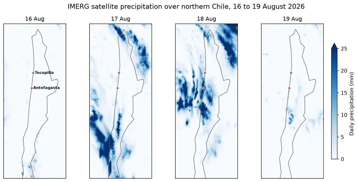
The 16th is essentially dry, a normal Atacama day. By the 17th a band of rain has arrived along the coast and against the Andes further east, exactly the two zones the earlier discussion of orographic lifting would predict. The 18th, the day Tocopilla flooded, shows the heaviest and most widespread rain of the four days, with a visible patch sitting right over the town itself, and by the 19th the system has largely pulled away, leaving only scattered showers behind. The double band running the length of every panel, one hugging the coast and one further inland, is the coastline on one side and the Andes on the other, the same two features that ordinarily keep this stretch of desert dry now channelling the rain that got through.
The El Niño connection
El Niño is the warm phase of ENSO, a natural, roughly three to seven year oscillation in sea surface temperature and air pressure across the tropical Pacific. By mid July 2026 the weekly Niño 3.4 index, the standard measure of that warming in the east central tropical Pacific, stood at about +2.1°C [9], and NOAA’s Climate Prediction Center put the odds of this event ranking among the strongest on record at around 90 percent in its August outlook [10]. This is shaping up to be one of the handful of truly strong El Niño winters on record for the Southern Hemisphere, in the company of 1982, 1997, and 2015.
El Niño does not reach Antofagasta by direct transport. Warm water off Peru does not simply drift south and rain out over the Atacama. It works through what is usually called a teleconnection, a link between weather in one part of the world and weather somewhere else, mediated by the atmosphere rather than by any physical connection between the two places. Unusually warm water in the tropical Pacific shifts where thunderstorms cluster along the equator, and that shift in tropical convection excites a chain of high and low pressure anomalies that propagates south and east across the Pacific and down over South America, a wave pattern meteorologists call the Pacific South America pattern, or PSA [6]. One common expression of the PSA pattern nudges the storm track, the belt of fronts and low pressure systems that in an ordinary year passes well south of the Atacama, further north than usual, and increases how often cutoff lows and atmospheric rivers reach the 20 to 30 degree south latitude band where Antofagasta and Tocopilla sit.
None of that guarantees any single storm. The PSA pattern is a shift in odds over a season, not a forecast for one Tuesday afternoon in August. But it is a real and reasonably well documented shift, and it is consistent with the fact that the strongest El Niño years on record, 1982, 1997, and 2015, are also the years that show up most often in the historical record of Atacama flood events. The number that makes the news
The 30 millimetre figure for Tocopilla comes from news reporting rather than an official gauge total published at time of writing, so it should be read as an approximate, order of magnitude number rather than a precise one. Even so, set against a long term annual average of about 5 millimetres, the ratio is the story:
Five weeks, three declarations
Lining the three events up on a single timeline shows something a single headline does not: the risk did not come out of nowhere. Chilean authorities flagged the elevated hazard in advance, twice, and the system that actually caused the damage at Tocopilla arrived two days after the preventive emergency window they had declared had already closed.
What the forecast ensembles were saying
The preventive emergency in the timeline above was based on human forecaster judgment applied to model guidance, not a single number. It is worth looking at what the guidance itself actually showed. Two operational centres run global ensemble forecasts every day: NOAA's GEFS, 31 members [11], and ECMWF's IFS ENS, 51 members [12], a control run plus perturbed members that sample how small differences in the starting state and the model itself grow into different outcomes days later. dynamical.org republishes both as public, analysis ready Zarr archives on AWS, forecasts included, going back to 2020 for GEFS and 2024 for IFS ENS, which makes it possible to pull the actual archived ensemble forecasts for Tocopilla rather than relying on a summary after the fact.
LAT, LON = -22.0919, -70.1979  # Tocopilla, Chile
EVENT_START = pd.Timestamp("2026-08-18T00:00:00")
EVENT_END = pd.Timestamp("2026-08-19T00:00:00")
INIT_TIMES = ["2026-08-14T00", "2026-08-15T00", "2026-08-16T00",
              "2026-08-17T00", "2026-08-18T00"]


def open_icechunk(bucket, prefix):
    storage = icechunk.s3_storage(bucket=bucket, prefix=prefix,
                                   region="us-west-2", anonymous=True)
    repo = icechunk.Repository.open(storage)
    session = repo.readonly_session("main")
    return xr.open_zarr(session.store, chunks=None, consolidated=False)


def accumulated_precip_mm(ds, init_time):
    """24h accumulated precipitation (mm) at the grid cell nearest Tocopilla,
    one value per ensemble member, for the given forecast init_time."""
    point = ds["precipitation_surface"].sel(
        init_time=init_time, latitude=LAT, longitude=LON, method="nearest")
    valid_time = ds["valid_time"].sel(init_time=init_time)
    in_window = (valid_time >= EVENT_START) & (valid_time < EVENT_END)
    point = point.sel(lead_time=point["lead_time"][in_window.values])
    # precipitation_surface is an average rate (mm/s) since the previous
    # 3 hourly step; multiplying by the step length and summing gives mm.
    return (point * 3 * 3600).sum(dim="lead_time").values
Each forecast is pulled fresh from the archive, converted from an average precipitation rate per 3 hour step into millimetres accumulated over the calendar day of 18 August, and cached locally so it renders again without downloading anything a second time:
CACHE_PATH = "data/tocopilla_ensemble_precip.csv"

if os.path.exists(CACHE_PATH):
    ens_df = pd.read_csv(CACHE_PATH)
else:
    sources = {
        "GEFS": ("dynamical-noaa-gefs", "noaa-gefs-forecast-35-day/v0.2.0.icechunk"),
        "IFS ENS": ("dynamical-ecmwf-ifs-ens",
                    "ecmwf-ifs-ens-forecast-15-day-0-25-degree/v0.1.0.icechunk"),
    }
    rows = []
    for model, (bucket, prefix) in sources.items():
        ds = open_icechunk(bucket, prefix)
        for init in INIT_TIMES:
            lead_days = (EVENT_START - pd.Timestamp(init)).days
            for member, mm in enumerate(accumulated_precip_mm(ds, init)):
                rows.append({"model": model, "lead_days": lead_days,
                             "ensemble_member": member, "precip_mm": float(mm)})
    ens_df = pd.DataFrame(rows)
    ens_df.to_csv(CACHE_PATH, index=False)

ens_df.groupby(["model", "lead_days"])["precip_mm"].median()

COLOR_GEFS, COLOR_IFSENS, COLOR_OBS = "#4c72b0", "#dd8452", "#c44e52"
OBS_MM = 30  # approximate, reported figure, see caveats below

lead_order = sorted(ens_df["lead_days"].unique(), reverse=True)
rng = np.random.default_rng(0)

fig, ax = plt.subplots(figsize=(8.5, 5.5))
width = 0.32
for i, lead in enumerate(lead_order):
    for j, (model, color) in enumerate([("GEFS", COLOR_GEFS), ("IFS ENS", COLOR_IFSENS)]):
        vals = ens_df.loc[(ens_df["lead_days"] == lead) & (ens_df["model"] == model),
                           "precip_mm"].values
        x0 = i + (j - 0.5) * width * 1.15
        ax.boxplot(vals, positions=[x0], widths=width, patch_artist=True, showfliers=False,
                   medianprops=dict(color="black", linewidth=1.4),
                   boxprops=dict(facecolor=color, alpha=0.55, edgecolor=color),
                   whiskerprops=dict(color=color), capprops=dict(color=color))
        jitter = rng.uniform(-width * 0.32, width * 0.32, size=len(vals))
        ax.scatter(x0 + jitter, vals, color=color, s=9, alpha=0.5, zorder=3)

ax.axhline(OBS_MM, color=COLOR_OBS, linestyle="--", linewidth=1.4, zorder=4)
ax.text(len(lead_order) - 0.55, OBS_MM + 1.2, "~30 mm reported at Tocopilla",
        color=COLOR_OBS, fontsize=9, ha="right")

ax.set_xticks(range(len(lead_order)))
ax.set_xticklabels([f"{d} day{'s' if d != 1 else ''} ahead" if d else "same day"
                     for d in lead_order])
ax.set_ylabel("24h accumulated precipitation (mm)\nnearest grid cell to Tocopilla")
ax.set_title("GEFS vs. IFS ENS: forecast rain for 18 Aug 2026 at Tocopilla")
handles = [
    plt.Line2D([0], [0], color=COLOR_GEFS, lw=7, alpha=0.55, label="GEFS (31 members)"),
    plt.Line2D([0], [0], color=COLOR_IFSENS, lw=7, alpha=0.55, label="IFS ENS (51 members)"),
]
ax.legend(handles=handles, loc="upper left", fontsize=9)
ax.spines[["top", "right"]].set_visible(False)
fig.tight_layout()
fig.savefig("images/tocopilla_ensemble_precip.png", dpi=150)
plt.show()
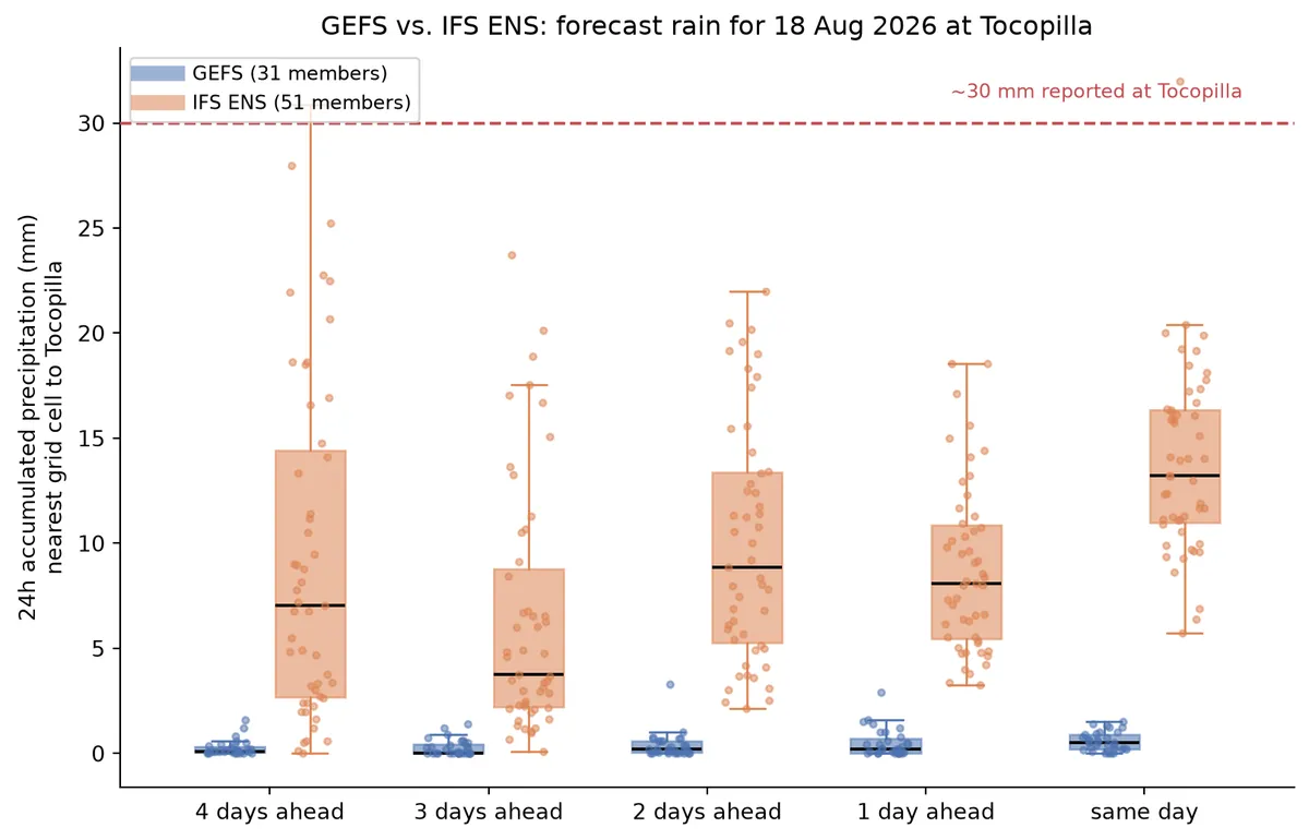
The two ensembles told noticeably different stories. GEFS stayed dry at this grid cell across every lead time shown, its median never climbing much past half a millimetre and its wettest member, out of 31, never reaching even 3.5 millimetres, right up to the forecast issued the morning of the event itself. IFS ENS carried real signal from four days out, with a median in the high single digits of millimetres and individual members already reaching into the twenties, and that signal grew both wetter and tighter as the event approached, with its shortest range median climbing above 13 millimetres and several members closing in on the reported total. Neither ensemble nailed the number, but one of the two was pointing at a genuinely wet, disruptive day well before it arrived, and the other essentially was not.
That gap between two operational centres forecasting the same point on the same day is what ensemble uncertainty means in practice for a case like this. It is not only about how spread out one model's own members are, it is also about whether the major forecasting centres agree there is a real signal at all, which is a harder problem for forecasters and emergency planners to act on than a single model simply being unsure of itself.
What this connection does and doesn't tell us
A few things worth being explicit about, since it is easy to overstate a seasonal pattern into something it isn't:
- El Niño shifts the odds of storms reaching this stretch of coast over a whole season. It does not cause, in any direct sense, a specific cutoff low on a specific Monday. Attributing one storm to El Niño with any precision requires a formal event attribution study, comparing simulations with and without the observed ocean warming, not just a seasonal correlation.
- Cutoff lows and atmospheric rivers reach the Atacama in non El Niño years too, 2015 among them. A strong El Niño raises the frequency, it does not invent the mechanism.
- The 30 mm figure for Tocopilla is a reported estimate, not a verified gauge total, and the death and displacement counts for both events were still being revised as search and cleanup continued at the time of writing. Treat the specific numbers here as a snapshot, not a final tally.
- None of this is a hazard forecast for the rest of the 2026 to 2027 El Niño season. A strong El Niño raises the odds of more events like these reaching northern Chile before the event ends, it does not say when or exactly where the next one lands.
- The ensemble comparison above uses a single 0.25 degree grid cell about 12 kilometres from Tocopilla, at coarse global model resolution, to stand in for a small coastal town squeezed between the ocean and a steep escarpment. Coarse global ensembles are known to struggle with exactly this kind of localised, terrain driven rainfall, which likely explains part of why even IFS ENS undershot the reported total. One event and five forecast issue times is a case study, not a verification study, and should not be read as a general claim that ECMWF’s model always outdoes NOAA’s for events like this one, only that it clearly did for this one.
- The IMERG panels are a satellite retrieval, not a rain gauge, and retrieval algorithms are known to carry more uncertainty over steep coastal terrain like Tocopilla’s escarpment than over open ocean or flat land. The Late Run used here is a low latency product, not the fully reprocessed research grade version NASA eventually releases, and the daily totals are summed over UTC calendar days rather than the local afternoon window the reporting describes, so the maps are a good guide to where and roughly when the rain fell, not a substitute for a calibrated gauge reading at Tocopilla itself.
The desert remembers
The Atacama's hyper aridity is why a flood there is newsworthy in a way a similar rainfall in Valdivia or Puerto Montt never would be, and it is also why a flood there does real damage out of proportion to the millimetres involved: decades without rain leave hillsides bare and drainage channels dry and inactive, so when the water does arrive it has nothing to slow it down. That is the same vulnerability that made 1997, and 1982, and 2015 into flood years worth naming individually in Chile’s climate record. A strong El Niño does not change the desert’s geography, its ocean current, or its mountains. It just shifts, for a season, how often the systems that can beat all three of those defenses show up. On the evidence of five weeks in 2026, this looks like one of the seasons where they show up more than most.
References
- Watch: Eyewitness video shows severe flooding in northern Chile after heavy rains, The Manila Times
- Chile Declares a Disaster Zone After Rain Hits the Driest Desert, The Rio Times
- Chile State of Catastrophe: 100,000 Cut Off by Floods, The Rio Times
- Chile Declares a Preventive Weather Emergency Across Five Northern Regions, The Rio Times
- Weeklong rainstorms in Chile blamed on El Nino kill at least 10 and trigger flash floods, WLRN/AP
- Rain Where It Shouldn't Fall: El Niño and Chile's Deadly Winter Floods, IAMElNino.com
- Flooding in Chile's Atacama Desert after years' worth of rain in one day, NOAA Climate.gov
- Atmospheric Rivers Swamp Central Chile, NASA Earth Observatory
- Relative Oceanic Nino Index and Nino3.4 Data, Brian McNoldy / University of Miami
- NOAA: El Niño has 69% chance of reaching historic strength later this year, Fox Weather
- NOAA GEFS forecast, 35 day, dynamical.org
- ECMWF IFS ENS forecast, 15 day, 0.25 degree, dynamical.org
- NASA IMERG analysis, late, dynamical.org