Making decisions with uncertainty
Recently, I had a discussion with a colleague about using traffic data—such as road temperature and road conditions (e.g., is it snowing or raining)—to make decisions on when to send trucks to clean the roads. This conversation reminded me of a Python library I came across some time ago, called mcda, which is designed for Multi-Criteria Decision Aiding (MCDA). MCDA is a framework for making decisions based on multiple, often conflicting, criteria. I didn’t know much about this topic before, but this piqued my curiosity to dig a bit further into how such a framework can help make well-informed decisions.
MCDA is a structured approach to decision-making that helps individuals or groups evaluate and choose between multiple options when faced with multiple, potentially conflicting, objectives or criteria. It’s particularly useful when dealing with complex decisions where a simple ranking or single criterion isn’t sufficient. This is exactly what’s needed for scenarios like the one I described above.
How MCDA Works
MCDA typically involves several key steps:
- Selection of relevant criteria and subcriteria: These are the aspects or features that matter for the decision (e.g., road temperature, precipitation, traffic volume).
- Assignment of weights: Each criterion is given a weight reflecting its importance in the decision-making process.
- Normalization: Since criteria may be measured on different scales (e.g., temperature in degrees, precipitation in mm), normalization brings all data to a common scale.
- Aggregation: The normalized and weighted criteria are combined using mathematical functions to produce a single score for each alternative.
- Sensitivity and robustness analysis: Since results can be sensitive to the choice of weights, normalization, and aggregation methods—as well as uncertainty in the data—MCDA often includes analysis to test how robust the results are to these factors.
MCDA is widely used in fields like environmental assessment, sustainability, healthcare, and risk analysis, where decisions are complex and must balance multiple objectives.
Applying MCDA to Road Maintenance Decisions
Let’s return to the road maintenance scenario. Imagine you have to decide when and where to send snowplows or salt trucks during winter. The decision depends on several factors:
- Road temperature: Lower temperatures may require more urgent action.
- Precipitation: Is it snowing, raining, or freezing rain?
- Traffic volume: High-traffic roads may be prioritized.
- Forecast uncertainty: Weather predictions are never 100% certain.
Using MCDA, you can:
- Define your criteria: For example, road temperature, precipitation type, traffic volume, and forecast confidence.
- Assign weights: Maybe road temperature and precipitation type are most important, so they get higher weights.
- Normalize your data: Convert all measurements to a 0–1 scale.
- Aggregate scores: Combine the normalized, weighted scores for each road segment.
- Analyze sensitivity: See how changes in weights or data uncertainty affect your decisions.
Example: Deciding When to Deploy Road Maintenance Trucks
Suppose you have the following data for three road segments:
| Road Segment | Temperature (°C) | Precipitation (mm/hr) | Traffic Volume (cars/hr) | Forecast Confidence (%) |
|---|---|---|---|---|
| A | -5 | 2 | 500 | 80 |
| B | -2 | 0 | 1000 | 60 |
| C | -8 | 1 | 300 | 90 |
You decide that temperature and precipitation are most important (weight = 0.4 each), traffic volume is less important (weight = 0.15), and forecast confidence is least important (weight = 0.05).
Minimal Working Example with mcda
Below is a minimal, self-contained example using only the mcda library. This example shows how to set up the decision matrix, define scales and weights, normalize the data, aggregate the scores, dump the results to a CSV file, and plot the results.
from mcda import PerformanceTable, normalize
from mcda.scales import QuantitativeScale, MIN, MAX
from mcda.mavt.aggregators import WeightedSum
import pandas as pd
import matplotlib.pyplot as plt
# Define alternatives and criteria
alternatives = ['A', 'B', 'C']
criteria = ['Temperature', 'Precipitation', 'Traffic', 'Confidence']
# Define the performance table (rows: alternatives, columns: criteria)
data = [
[-5, 2, 500, 80], # A
[-2, 0, 1000, 60], # B
[-8, 1, 300, 90] # C
]
# Define scales for each criterion
scales = {
'Temperature': QuantitativeScale(-10, 0, preference_direction=MIN), # Lower is better
'Precipitation': QuantitativeScale(0, 5, preference_direction=MAX), # Higher is better
'Traffic': QuantitativeScale(0, 2000, preference_direction=MAX), # Higher is better
'Confidence': QuantitativeScale(0, 100, preference_direction=MIN) # Lower is better
}
# Create the performance table
performance_table = PerformanceTable(
data,
alternatives=alternatives,
criteria=criteria,
scales=scales
)
# Define weights for each criterion
criteria_weights = {
'Temperature': 0.4,
'Precipitation': 0.4,
'Traffic': 0.15,
'Confidence': 0.05
}
# Create the weighted sum aggregator
weighted_sum = WeightedSum(criteria_weights)
# Normalize the performance table
normalized_table = normalize(performance_table)
# Compute the scores
scores = weighted_sum(normalized_table)
scores_df = scores.data.reset_index()
scores_df.columns = ['Road_Segment', 'Score']
# Save results to CSV
scores_df.to_csv('mcda_results.csv', index=False)
print("Results saved to mcda_results.csv")
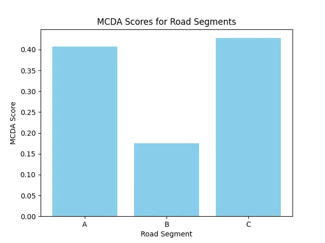
# Plot the results
plt.bar(scores_df['Road_Segment'], scores_df['Score'], color='skyblue')
plt.xlabel('Road Segment')
plt.ylabel('MCDA Score')
plt.title('MCDA Scores for Road Segments')
plt.show()
What this does:
- Sets up the alternatives and their values.
- Defines the criteria, their weights, and whether higher or lower values are better.
- Normalizes the data using the built-in
normalizefunction. - Aggregates the normalized values using the Weighted Sum Model.
- Saves the results to a CSV file (
mcda_results.csv). - Plots the scores for each road segment.
Incorporating Uncertainty in MCDA
In real-world decision-making, our data and weights are rarely exact. For example, weather forecasts come with confidence intervals, sensor measurements have errors, and the importance of each criterion may be debated among stakeholders. MCDA can handle this uncertainty through simulation-based approaches.
Understanding Sources of Uncertainty
Uncertainty can enter the MCDA process in several ways:
- Data uncertainty: Measurements like temperature or precipitation may have measurement errors or be forecasts with confidence intervals.
- Weight uncertainty: The relative importance of criteria may not be precisely known.
- Model uncertainty: The choice of normalization or aggregation method can affect results.
Monte Carlo Simulation for Uncertainty Analysis
While the mcda library doesn't have built-in uncertainty modeling, we can implement Monte Carlo simulation by running the MCDA process many times with slightly different input values. This approach helps us understand how robust our decisions are to uncertainty in the inputs.
Here's an enhanced example that incorporates uncertainty in the forecast confidence values:
import numpy as np
import pandas as pd
import matplotlib.pyplot as plt
from mcda import PerformanceTable, normalize
from mcda.scales import QuantitativeScale, MIN, MAX
from mcda.mavt.aggregators import WeightedSum

# Set random seed for reproducibility
np.random.seed(42)

# Define alternatives and criteria (same as before)
alternatives = ['A', 'B', 'C']
criteria = ['Temperature', 'Precipitation', 'Traffic', 'Confidence']

# Base data with deterministic values for most criteria
base_data = [
    [-5, 2, 500, 80],   # A
    [-2, 0, 1000, 60],  # B
    [-8, 1, 300, 90]    # C
]

# Define uncertainty in forecast confidence (±10% standard deviation)
confidence_means = [80, 60, 90]
confidence_stds = [8, 6, 9]  # 10% of the mean values

# Define scales and weights (same as before)
scales = {
    'Temperature': QuantitativeScale(-10, 0, preference_direction=MIN),
    'Precipitation': QuantitativeScale(0, 5, preference_direction=MAX),
    'Traffic': QuantitativeScale(0, 2000, preference_direction=MAX),
    'Confidence': QuantitativeScale(0, 100, preference_direction=MIN)
}

criteria_weights = {
    'Temperature': 0.4,
    'Precipitation': 0.4,
    'Traffic': 0.15,
    'Confidence': 0.05
}

# Monte Carlo simulation
n_simulations = 1000
all_scores = []

for _ in range(n_simulations):
    # Sample new confidence values with uncertainty
    sampled_confidence = np.random.normal(confidence_means, confidence_stds)
    # Clip to valid range [0, 100]
    sampled_confidence = np.clip(sampled_confidence, 0, 100)

    # Create data with uncertain confidence values
    data_with_uncertainty = [
        [-5, 2, 500, sampled_confidence[0]],   # A
        [-2, 0, 1000, sampled_confidence[1]],  # B
        [-8, 1, 300, sampled_confidence[2]]    # C
    ]

    # Run MCDA process
    performance_table = PerformanceTable(
        data_with_uncertainty,
        alternatives=alternatives,
        criteria=criteria,
        scales=scales
    )

    weighted_sum = WeightedSum(criteria_weights)
    normalized_table = normalize(performance_table)
    scores = weighted_sum(normalized_table)

    # Store results
    all_scores.append(scores.data.values)

# Convert to numpy array for easier analysis
all_scores = np.array(all_scores)  # shape: (n_simulations, n_alternatives)

# Calculate statistics
mean_scores = np.mean(all_scores, axis=0)
std_scores = np.std(all_scores, axis=0)
percentile_5 = np.percentile(all_scores, 5, axis=0)
percentile_95 = np.percentile(all_scores, 95, axis=0)

# Create results DataFrame
results_df = pd.DataFrame({
    'Road_Segment': alternatives,
    'Mean_Score': mean_scores,
    'Std_Score': std_scores,
    'P5_Score': percentile_5,
    'P95_Score': percentile_95
})

print("MCDA Results with Uncertainty:")
print(results_df.round(3))

# Visualization: Boxplots showing uncertainty
fig, ax1 = plt.subplots(1, 1, figsize=(12, 5))

# Boxplot showing score distributions
# Convert to list of arrays, one for each alternative
boxplot_data = [all_scores[:, i] for i in range(len(alternatives))]
ax1.boxplot(boxplot_data, labels=alternatives)
ax1.set_xlabel('Road Segment')
ax1.set_ylabel('MCDA Score')
ax1.set_title('MCDA Scores with Uncertainty\n(Boxplots)')
ax1.grid(True, alpha=0.3)

plt.tight_layout()
plt.show()
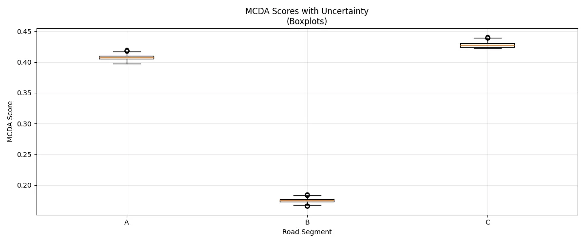
Interpreting Uncertainty Results
The uncertainty analysis provides several insights:
- Robustness of rankings: If the ranking of alternatives remains consistent across simulations, the decision is robust to the uncertainty considered.
- Confidence intervals: The 5th and 95th percentiles give us a 90% confidence interval for each alternative's score.
- Decision sensitivity: Large error bars or wide boxplots indicate that an alternative's score is sensitive to the uncertain inputs.
- Risk assessment: Understanding the range of possible outcomes helps in making more informed decisions under uncertainty.
Summary
The MCDA approach—and tools like mcda—provide a systematic way to make complex decisions using multiple, possibly uncertain, criteria. While the mcda library doesn't have built-in uncertainty modeling, we can easily implement Monte Carlo simulation to understand how uncertainty affects our decisions.
Whether you're managing road maintenance, choosing a project, or evaluating policy options, combining MCDA with uncertainty analysis helps you make more robust and informed decisions. The visualization of uncertainty through boxplots and error bars provides valuable insights into the reliability of your decision-making process.