Kriging of road surface temperatures: spatial interpolation

03 Jun, 2025

In this second part of the Kriging methodology series, we implement Universal Kriging to predict road surface temperatures at unknown locations using the data preparation described in the previous post. Universal Kriging extends ordinary kriging by incorporating spatial trends and covariates, making it ideal for road temperature modeling where terrain features significantly influence temperature patterns.

Required Libraries

We use the following Python libraries:

pandas and geopandas for data manipulation and spatial operations
pykrige - a comprehensive Kriging toolkit for Python
sklearn for feature preprocessing and scaling
sqlite3 for database operations
numpy for numerical computations

Data Loading and Preparation

Loading Meteorological Data

First, we load temperature and meteorological data from an SQLite database. The data is organized by year and variable type:

import sqlite3
import pandas as pd
import numpy as np
from pykrige.uk import UniversalKriging
from sklearn.preprocessing import StandardScaler
from datetime import datetime

def load_and_merge_data_optimized(variables, year):
    """
    Load data from SQLite databases and merge into a single dataframe.

    Args:
        variables: List of meteorological variables to load
        year: Year of data to load

    Returns:
        DataFrame with merged data from all variables
    """
    dataframes = []

    for variable in variables:
        db_path = os.path.join(DB, f'OBSTABLE_{variable}_{year}.sqlite')
        if not os.path.exists(db_path):
            print(f"Warning: Database file not found: {db_path}")
            continue

        conn = sqlite3.connect(db_path)
        # Optimize SQLite performance
        conn.execute('PRAGMA synchronous = OFF')
        conn.execute('PRAGMA journal_mode = MEMORY')

        query = f"SELECT valid_dttm, SID, lat, lon, {variable} FROM SYNOP"

        try:
            for chunk in pd.read_sql_query(query, conn, chunksize=10000):
                dataframes.append(chunk)
        except sqlite3.Error as e:
            print(f"SQLite error when reading {variable}: {e}")
        finally:
            conn.close()

    if not dataframes:
        raise ValueError("No data loaded from database")

    # Merge all dataframes and remove duplicates
    full_df = pd.concat(dataframes, ignore_index=True)
    merged_df = full_df.groupby(['valid_dttm', 'SID', 'lat', 'lon']).first().reset_index()
    return merged_df

# Configuration
DB = "./OBSTABLE"
variables = ['TROAD', 'T2m', 'Td2m', 'D10m', 'S10m', 'AccPcp12h']
year = 2023
date_chosen = datetime(year, 8, 11, 15)

# Load meteorological data
print("Loading meteorological data...")
df = load_and_merge_data_optimized(variables, year)

Integrating Terrain Covariates

Next, we merge the meteorological data with the terrain metrics calculated in the previous post. These orographic features (elevation, slope, aspect) serve as covariates in the Universal Kriging model:

# Load pre-processed terrain metrics
station_gis_metrics = pd.read_csv('../data/station_metrics.csv')

# Remove duplicate coordinate columns
columns_to_drop = ['lat', 'lon']
cleaned = station_gis_metrics.drop(columns=columns_to_drop)

# Merge datasets using station identifiers
merged = df.merge(
    cleaned,
    left_on='SID',           # Station ID in meteorological data
    right_on='station_id',   # Station ID in terrain data
    how='inner'
)

Temporal Filtering

We select a specific date for analysis. The choice of date can significantly impact kriging performance due to varying meteorological conditions:

# Convert timestamps and filter for specific date
merged["dates"] = pd.to_datetime(merged["valid_dttm"], unit="s")
df = merged[merged["dates"] == date_chosen]

print(f"Selected {len(df)} stations for date: {date_chosen}")

Universal Kriging Implementation

Feature Preparation and Scaling

Universal Kriging requires careful preparation of coordinates, target values, and covariates:

# Extract coordinates and target variable
coords = df[['lon', 'lat']].values
values = df['TROAD'].values

# Select terrain covariates
covariates = ['elev_m', 'slope_deg', 'aspect_deg']
X = df[covariates].values

# Standardize covariates for numerical stability
scaler = StandardScaler()
X_scaled = scaler.fit_transform(X)

print(f"Using {len(covariates)} covariates: {covariates}")
print(f"Temperature range: {values.min():.1f}°C to {values.max():.1f}°C")

Model Fitting

The Universal Kriging model incorporates the scaled covariates as specified drift terms:

# Fit Universal Kriging model
UK = UniversalKriging(
    df['lon'], df['lat'], df['TROAD'],
    drift_terms=['specified'],
    specified_drift=[X_scaled[:, i] for i in range(X_scaled.shape[1])],
    variogram_model='exponential',
    verbose=True,
    enable_plotting=False
)

print(f"Fitted variogram parameters:")
print(f"  Sill: {UK.variogram_model_parameters[0]:.3f}")
print(f"  Range: {UK.variogram_model_parameters[1]:.3f}")
print(f"  Nugget: {UK.variogram_model_parameters[2]:.3f}")

The variogram parameters provide insights into spatial correlation:

Sill: Total variance in the data
Range: Distance beyond which observations are uncorrelated
Nugget: Measurement error or micro-scale variation

Temperature Prediction

Point Predictions

For discrete point predictions at specific locations we need to calculate again the terrain metrics calculated in the previous post, but for the points where we want to use kriging. These are saved in the file below:

new_points = pd.read_csv('../data/station_metrics_kriging_points.csv')
print(f"Loaded {len(new_points)} prediction points")

# Prepare prediction coordinates and covariates
pred_coords = new_points[['lon', 'lat']].values
X_pred = new_points[covariates].values

# Apply same scaling as training data
X_pred_scaled = scaler.transform(X_pred)

# Perform predictions
pred_troad, pred_var = UK.execute(
    'points',
    pred_coords[:, 0],
    pred_coords[:, 1],
    specified_drift_arrays=[X_pred_scaled[:, i] for i in range(X_pred_scaled.shape[1])]
)

# Store results
new_points['TROAD_predicted'] = pred_troad
new_points['TROAD_variance'] = pred_var

print(f"Prediction complete. Mean predicted temperature: {pred_troad.mean():.1f}°C")
print(f"Prediction uncertainty range: {pred_var.min():.3f} to {pred_var.max():.3f}")

Continuous Surface Mapping

In order to visualize the results we can create a continuous temperature surface. To do this, we first generate a regular grid and interpolate the covariates to this grid:

    """Create regular grid for continuous mapping"""
    min_lon, min_lat, max_lon, max_lat = bounds
    lon_grid = np.arange(min_lon, max_lon + resolution, resolution)
    lat_grid = np.arange(min_lat, max_lat + resolution, resolution)
    lon_mesh, lat_mesh = np.meshgrid(lon_grid, lat_grid)
    grid_coords = np.column_stack([lon_mesh.ravel(), lat_mesh.ravel()])
    return grid_coords, lon_mesh.shape

def interpolate_covariates_for_grid(grid_coords, station_coords, station_covariates):
    """Interpolate covariates to grid points using nearest neighbor"""
    from scipy.spatial import cKDTree
    tree = cKDTree(station_coords)
    distances, indices = tree.query(grid_coords)
    return station_covariates[indices]

# Define prediction domain
bounds = (df['lon'].min() - 0.1, df['lat'].min() - 0.1,
          df['lon'].max() + 0.1, df['lat'].max() + 0.1)

# Create prediction grid
grid_coords, grid_shape = create_prediction_grid(bounds, resolution=0.05)
print(f"Created grid: {len(grid_coords)} points ({grid_shape[0]}×{grid_shape[1]})")

# Interpolate covariates and predict
grid_covariates = interpolate_covariates_for_grid(grid_coords, coords, X)
grid_covariates_scaled = scaler.transform(grid_covariates)

grid_predictions, grid_variance = UK.execute(
    'points',
    grid_coords[:, 0],
    grid_coords[:, 1],
    specified_drift_arrays=[grid_covariates_scaled[:, i] for i in range(grid_covariates_scaled.shape[1])]
)

The whole procedure can found in this script.

Some results

Finally, we test the above implementation on some specific dates. The plot below shows the results for the 11th of February 2023 over a region in Jylland.

predictions_kriging_202302

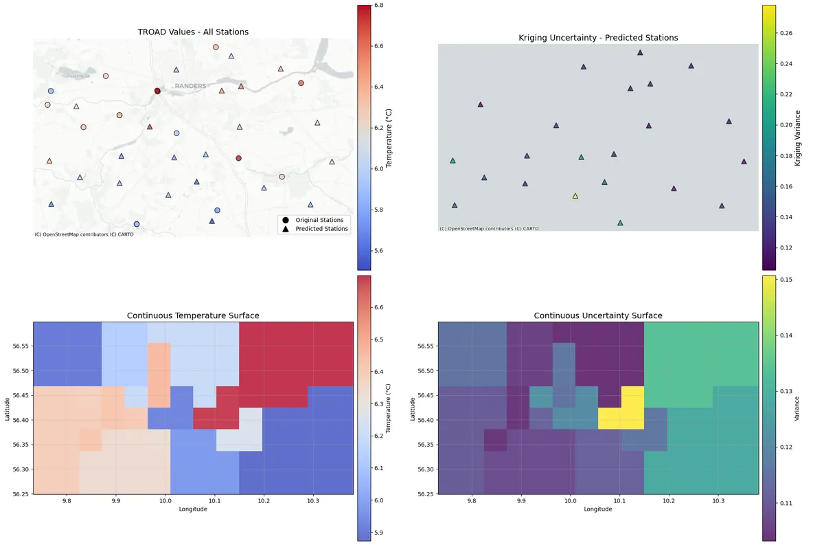
From the continuous temperature maps, the color scale appears to span a relatively small range of roughly 2-3°C. For a spatial domain that covers an area of a few hundred kilometers, this suggests that the kriging is producing overly smooth predictions, local spatial patterns aren't being well captured and the interpolation is "pulling" values toward the global mean.

The continuous surface shows very gradual, smooth transitions rather than sharp gradients one wouldl expect near topographic features Local hot/cold spots related to microclimates. Despite using elevation, slope, and aspect as covariates, the predicted surface doesn't show strong correlation with expected topographic effects (e.g., clear elevation-temperature relationships).

Testing on another date, this time during the 11th of August 2023.

predictions_kriging_202308

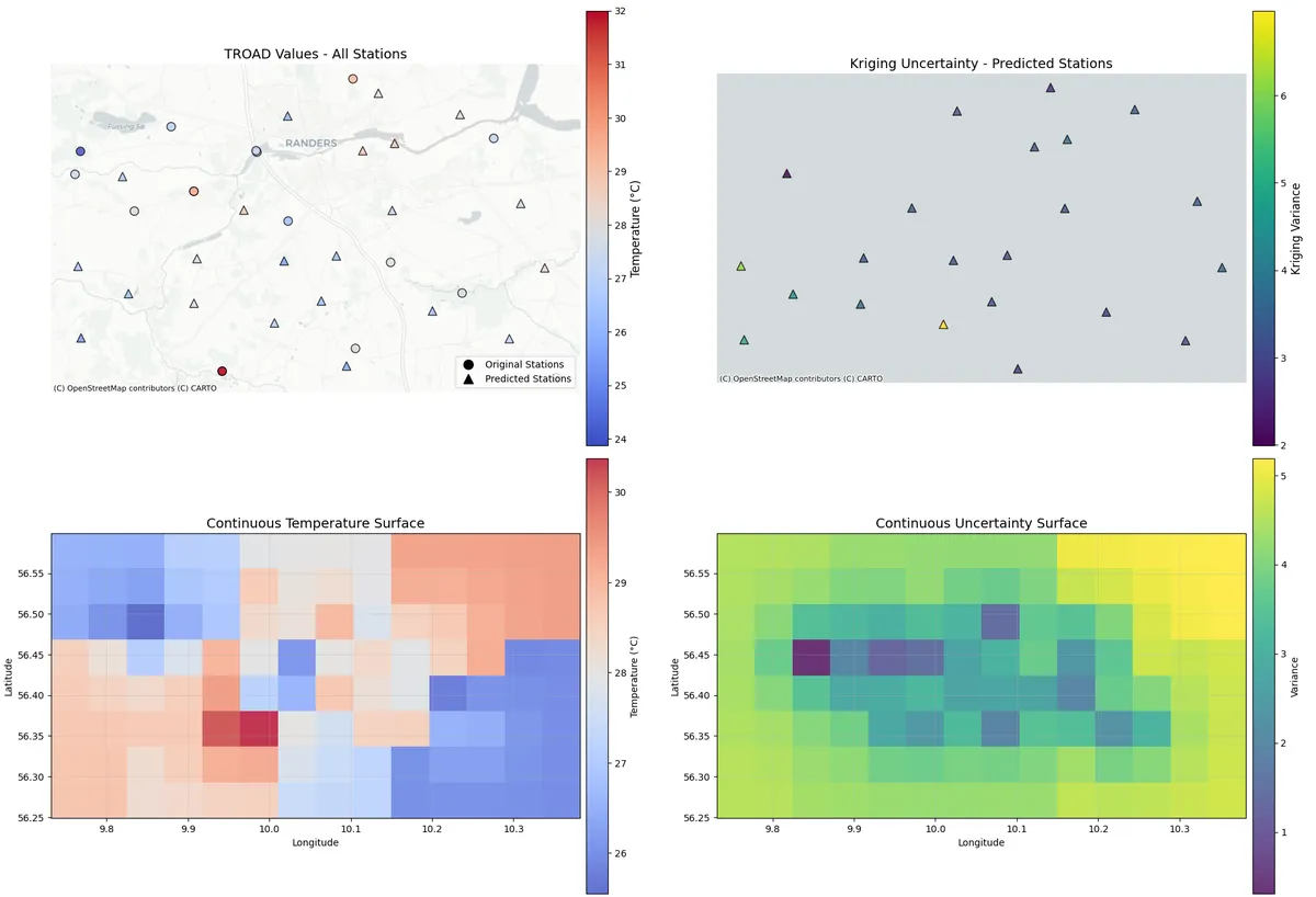
The August results show dramatically better performance compared to the February case. This reveals several important insights:

Much Improved Spatial Variation

Larger Temperature Range. August: ~7°C range (24-31°C) vs January: ~3°C range. This larger signal-to-noise ratio makes spatial patterns much more detectable
Clear Spatial Structure. The continuous temperature surface now shows distinct hot and cold regions rather than smooth gradients. Sharp temperature boundaries indicate real spatial features and coherent spatial patterns that suggest meaningful physical processes
Realistic Temperature Distribution. Clear east-west gradient (cooler in the east, warmer in the west) and localized hot spots that could correspond to urban areas or specific land use. Spatial clustering of similar temperatures

The uncertainty is reduced as well.

Lower Variance Values. August uncertainty ranges ~1-5 units vs higher values in February. More confident predictions are due to stronger spatial signal.
Spatial Structure in Uncertainty. Lower uncertainty in areas with strong temperature gradients (where the signal is clear). Higher uncertainty in transition zones (more realistic). This particular date produces an heterogeneous uncertainty pattern rather than uniform.

This suggest that this simple Kriging approach is highly season-dependent:

Summer: Strong spatial patterns, good predictions

Winter: Weak patterns, high uncertainty.

One way to make the kriging predictions more realistic is to include extra weather information from a numerical weather model. This could potentially provide the realistic large-scale patterns that the sparse station network can't capture, allowing kriging to focus on local corrections and fine-scale features.