From weather analogs to diffusion models
At the end of 2022 you could count the machine learning weather models on the fingers of one hand: FourCastNet, Keisler's graph network, Pangu-Weather and GraphCast. They had a lot in common. All of them were global, all were trained on ERA5 (ECMWF's reconstruction of the weather since 1940), all were deterministic (one input, one forecast), and all borrowed their architecture from computer vision or graph learning: vision transformers, Fourier neural operators, graph neural networks.
Four years later there are too many to count. There are regional models, ensemble models, nowcasting models, models that go straight from observations to forecasts, and people now talk about foundation models of the atmosphere: large models trained once on many kinds of data and then adapted to different tasks. Microsoft's Aurora is one example. Another is WeatherGenerator, an EU-funded project coordinated by ECMWF that is building a machine learning Earth system model trained on reanalyses, forecast data and observations (https://github.com/ecmwf/WeatherGenerator). For a sense of scale, see this curated list: https://github.com/shengchaochen82/Awesome-Foundation-Models-for-Weather-and-Climate.
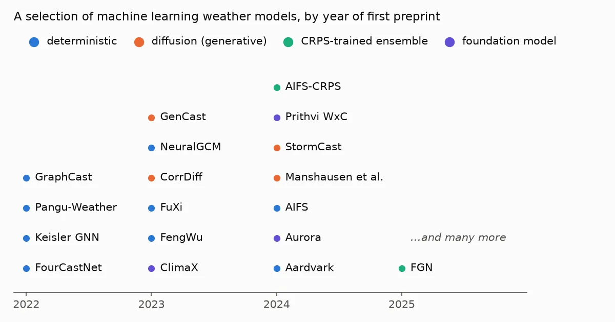 A selection of machine learning weather models by year of first preprint, coloured by type
With so many names around it is easy to lose track of what actually differs between them, so I want to write a short refresher on the fundamentals. I start with diffusion models. Not because they came first (they did not), but because the idea behind them is the easiest to picture.
One clarification first. "Diffusion", "transformer" and "graph network" are not three competing kinds of model. Transformers and graph networks are architectures: the shape of the network. Diffusion is a way of training and using a network: instead of predicting one answer, it learns to draw samples from a distribution. Many diffusion weather models have a transformer or a graph network inside; GenCast, for example, is a diffusion model built on a graph transformer. The more useful split is between models that predict the single most likely next state and models that learn what the weather can look like and draw from it. This post is about the second kind, and it starts from an idea forecasters have used for decades: look at what the weather has done before.
In this post I go from that old idea, through the image generators, to a recent paper by an NVIDIA team that uses a diffusion model to draw a full km-scale weather map from a handful of weather stations [1].
The oldest trick: find a day like today
Long before machine learning, forecasters asked a simple question: when did the weather last look like this, and what happened next? This is the analog method. Lorenz used naturally occurring analogs in 1969 to estimate how predictable the atmosphere is [2], and analog methods are still used today to correct model output, for example by searching past forecasts for ones that resemble today's and looking at what was actually observed [3].
Analogs have a hard limit. The atmosphere almost never repeats itself, so the closest past day is usually not that close. And you can only ever get back something that already happened.
Learning the weather from past data instead of solving the equations is not a new ambition either. In the 1950s statistical forecasting was a major research topic, and some forecasters believed that linear regression on today's weather would do at least as well as numerical models ever could [4]. Lorenz, put in charge of a statistical forecasting project at MIT, doubted it. He tested the idea on a small model of the atmosphere, 12 equations run on an early desk computer: the solutions never repeated themselves, and regression could only reproduce them poorly [4, 5]. While rerunning one of those simulations in 1961 from slightly rounded numbers, he got a completely different result, and that is how chaos was found. Physics won the first round, partly because the statistical tools of the time were linear and the data and computers were small.
Today's machine learning models are, in a sense, the second round. A neural network is a statistical model too, but a very nonlinear one, trained on decades of reanalysis on hardware nobody had in the 1950s. And the generative models in this post go one step further than predicting one number from others.
Now imagine instead that you could look at every past weather map at once, learn what weather in general looks like (how fronts curve, how rain cells cluster, how wind changes around a thunderstorm), and then draw a new map that never happened but could have. That is what a generative model does. It does not retrieve a past situation. It learns the distribution of past situations and samples from it.
How diffusion came to be
The method behind Stable Diffusion is called diffusion, and its history is short:
- 2015. Sohl-Dickstein and colleagues borrow an idea from physics: gradually destroy the structure in data by adding noise, then train a network to undo it step by step [6]. Interesting, but the pictures are poor.
- 2019 to 2021. Song and Ermon, and Ho and colleagues, make it work. Ho et al.'s denoising diffusion probabilistic models (DDPM) produce images as good as the best GANs of the time [7]. Song et al. show that all these variants are the same thing seen from different angles: learning the score, the direction in which data becomes more probable [8].
- 2022. The breakout year. DALL-E 2, Imagen and Stable Diffusion appear. Stable Diffusion's trick is to run the diffusion in a compressed "latent" space instead of on raw pixels, which makes it cheap enough to run on a home graphics card, and to steer it with text [9]. The same year, Karras and colleagues at NVIDIA publish EDM, a careful cleanup of the whole design space: how to schedule the noise, how to scale the network, how many steps to take [10]. EDM is the recipe almost all of NVIDIA's weather models use.
The idea in plain words:
- Take a real picture.
- Add some random noise to it, a little or a lot.
- Train a network to recover the clean picture from the noisy one.
- Repeat for millions of pictures and every amount of noise.
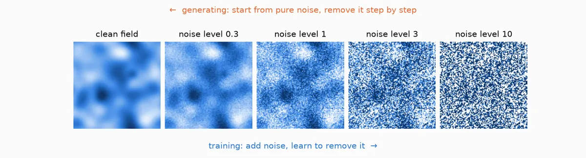 A synthetic weather-like field with increasing amounts of noise added. Training goes left to right, generating goes right to left.
The network only ever learns to denoise. But to remove noise well it has to know what real pictures look like, which shapes belong and which are noise. To make a new picture you start from pure noise and denoise in small steps, a few dozen times. Each step uses the network to nudge the picture towards "more like real data". A different starting noise gives a different picture.
To control what gets drawn, you give the network extra input while it denoises. In Stable Diffusion that input is your text prompt. In weather it can be a coarse global forecast, the current state of the atmosphere, or, as we will see, a list of weather station readings.
From pictures to weather maps
To a neural network a weather field looks a lot like an image: a grid of numbers. Temperature, wind components and precipitation are just channels, like red, green and blue, except there may be dozens of them. So it was natural to try the image machinery on weather, and from 2023 it took off:
- CorrDiff (NVIDIA, 2023) takes coarse 25 km ERA5 fields and generates 2 km fields over Taiwan, including radar reflectivity, a variable that is not even in the input [11].
- GenCast (Google DeepMind, 2023, published in Nature in 2025) does global medium-range ensemble forecasts with a diffusion model, and beats ECMWF's operational ensemble on 97% of the targets it was evaluated on [12].
- StormCast (NVIDIA, 2024) forecasts the weather hour by hour at 3 km over the central US, emulating NOAA's HRRR model, with realistic thunderstorms, cold pools and gust fronts [13].
Why bother, when deterministic models like GraphCast are already so good? Because of blur. A deterministic model trained to minimise squared error learns the average of all the futures that could happen. Averages are smooth: storms turn into blobs, peak winds and rain get underestimated, and it gets worse with lead time. A diffusion model does not average. Each sample is sharp, and if you want the uncertainty, you draw many samples and get an ensemble (a set of possible forecasts whose spread shows the uncertainty).
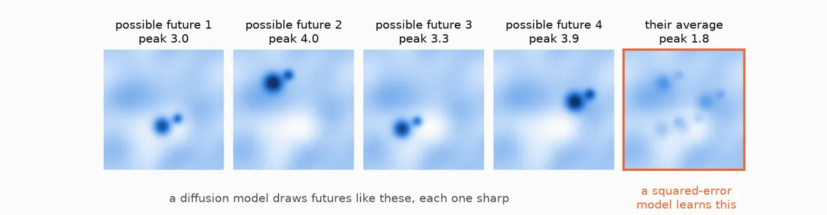 Toy example: four possible futures with a sharp rain cell in different places, and their average, where the cell is smeared out and its peak halve
Diffusion is not the only way out of the blur, though. Another route is to keep a model that produces a forecast in one pass, feed it some random noise so every run is different, and train it with a score that rewards a good ensemble instead of a good average, such as the continuous ranked probability score (CRPS). ECMWF's AIFS-CRPS [14] and Google DeepMind's FGN [15] work this way and also give sharp, skilful ensembles, at a fraction of the sampling cost. More on that in a later post.
The showcase: drawing a weather map from 40 stations
This is the paper I really want to talk about. Manshausen et al. (2025) [1] use diffusion not to forecast but for the step before the forecast: data assimilation.
To be clear from the start: nothing in this paper forecasts. The output is a 2D snapshot of the surface weather at one moment in time, the best guess of what the weather is right now given the stations. There is no time evolution in it. Moving that snapshot forward is a separate job for a forecast model (more on that in the Earth2Studio section below).
Every forecast needs an estimate of the current state of the atmosphere, called the analysis. Producing it means combining a short forecast with whatever observations are available, weighting each by how much you trust it. In operational regional models such as HRRR (NOAA's hourly 3 km model for the US) this is expensive and carefully tuned machinery.
The question in the paper: over a 384 x 384 km box in Oklahoma there are about 50 weather stations reporting wind and precipitation. The grid has 3 km spacing, so 128 x 128 = 16384 points per variable. Can you go from ~40 station readings to a realistic map of surface wind and rain?
You have far fewer numbers than unknowns, so the only way to fill the gaps is to know what weather usually looks like. Classical data assimilation writes this knowledge down by hand, as a background error covariance, and assumes it is Gaussian. The paper replaces that with a diffusion model that has learned it.
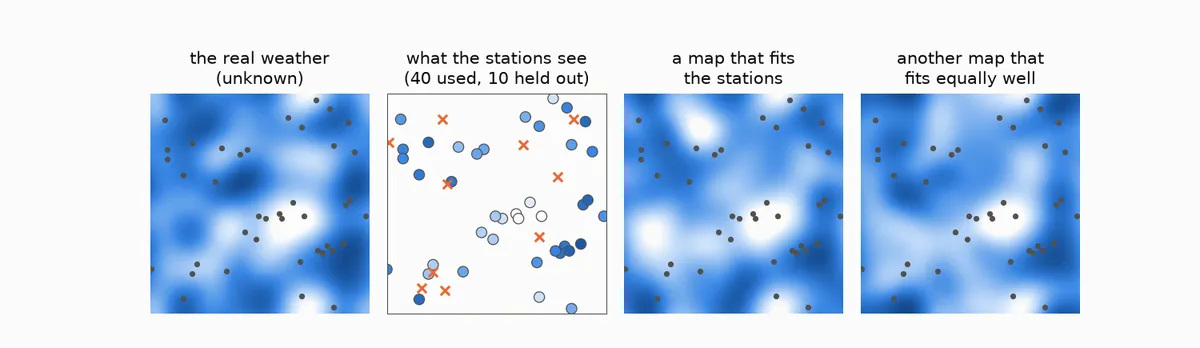 Toy example with a simple Gaussian prior, not the paper's model: a hidden field, the 40 stations that sample it (crosses are held-out stations), and two different maps that both agree with the stations
The figure shows the problem with a toy version. Many different maps agree with the same stations. Which ones you get depends entirely on what the model believes weather looks like between the stations. Here that belief is a simple smooth Gaussian; in the paper it is a diffusion model trained on millions of real maps, so the gaps get filled with fronts, rain cells and gust fronts instead of smooth blobs.
step 1: learn what the weather looks like
They train a diffusion model, with the EDM recipe, on about 2.5 million HRRR snapshots of three fields: the two surface wind components and precipitation. No prompt, no conditioning: the model just learns to generate plausible km-scale Oklahoma weather.
step 2: prompt it with the stations
If you have used the "fill in the missing part" tool of a photo editor, you already know the idea. Data assimilation of this kind is very close to inpainting: you know a few pixels (the stations) and ask the model to complete the rest of the picture so that it looks real and matches the pixels you know [16]. Diffusion models were already doing this with photos of bedrooms and faces in 2021 [8].
This is also where the Stable Diffusion analogy is closest. Instead of a text prompt, the prompt is the station readings. At every denoising step the map is pulled in two directions at once: towards "look like real weather", which is what the trained model knows, and towards "agree with the stations", which is added during sampling. The model guesses the clean map, checks it against the stations, and nudges the sample to reduce the mismatch. After a few dozen steps you have a map that is both realistic and consistent with the observations.
For the technically curious: the maths
This is Bayes' rule written in terms of scores:
grad log p(x | y) = grad log p(x) + grad log p(y | x)
where x is the full map and y the station readings. The first term is the learned score of the unconditional model. The second is the likelihood of the observations. If the observation operator A simply picks the grid points where the stations are, and the observation errors are Gaussian with standard deviation sigma, it is
grad log p(y | x) = A^T (y - A x) / sigma^2
that is, the mismatch at the stations spread back onto the grid. During sampling x is noisy, so the mismatch is computed on the denoiser's estimate of the clean map instead. This is score-based data assimilation [16], with the likelihood approximated as in diffusion posterior sampling [17].
The nice part: the model is trained once, without any observations. You can change which stations you use, or add new ones, without retraining. Just as Stable Diffusion was never trained on your particular prompt.
What they found
They tested on all of 2017, assimilating 40 stations and keeping 10 aside to check the result [1]:
It beats HRRR on the held-out stations. The ensemble mean has about 10% lower error (RMSE, root mean square error) than the HRRR analysis on stations it never saw [1]. HRRR is a full operational system using far more data.
It picked up relationships between variables nobody told it about. Give the model only east-west wind and rain at the stations, and it fills in north-south wind with gust fronts spreading out from the rain cells, as cold pools do [1]. That link between rain and wind was learned from the HRRR data. It is tempting to call this "learning physics", but I would not go that far: it is a joint statistical relationship that holds at a single instant, absorbed from a model (HRRR) that does have the physics. Whether models like this learn the dynamics, for example how small errors grow, is a different question, and the evidence so far says they mostly do not (I wrote about that in when AI models miss the butterfly).
It is fast. About 10 seconds per sample on one workstation GPU.
And what does not work yet [1]:
- The ensembles are underdispersive: members agree with each other more than they agree with reality. CorrDiff and StormCast show the same.
- Precipitation is biased low.
- Only three surface variables at one moment in time. No temperature, humidity, pressure, upper air, radar or satellite.
- The way the map is compared with the observations has to be simple. A nonlinear version for precipitation made the sampling blow up.
Dense or sparse: the spread tells you
Because you get an ensemble and not a single map, you also get a map of the uncertainty: where the members disagree, the stations did not pin the weather down. Close to a station the members agree; far from all stations they are free to differ. With more stations the whole map tightens.
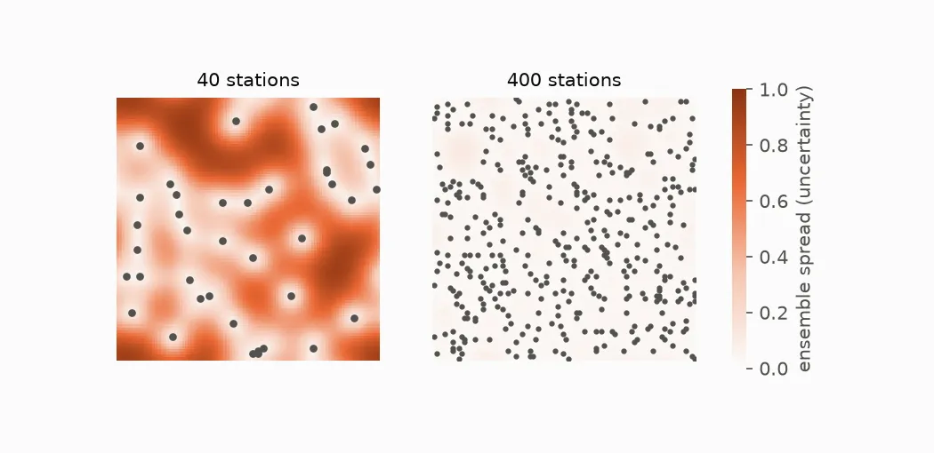 Toy example with the same Gaussian prior as above: ensemble spread with 40 stations is large away from the stations; with 400 stations it is small almost everywhere
What Earth2Studio actually ships
NVIDIA's Earth2Studio [18] is not a single model but a framework that runs
many, deterministic and generative. If you look in it for this paper, what
you find is StormCastSDA [19], and it is not quite the same thing. It is
the combination the paper's outlook asks for: a diffusion forecast model
with diffusion data assimilation attached. Instead of starting from nothing
every time, it takes the current weather, forecasts one hour ahead, and lets
whatever stations are reporting nudge that forecast while it is being drawn.
For the technically curious: how StormCastSDA works
From the code (commit 95f74e6, August 2026):
- The prior is StormCast [13], not an unconditional model. It takes the current 99-variable HRRR state plus 26 coarse global variables (from ERA5 or GFS) and predicts the state one hour later.
- It uses the CorrDiff split [11]. A deterministic network first predicts
the average next state; the diffusion model only draws the fine detail on
top. The station readings are converted to the same "detail" form
(
y_obs = y_obs - out) before they steer the sampling. - Two knobs control the steering:
sda_std_obs, how much error to assume in the observations (default 0.1 in normalised units), andsda_gamma, how hard to pull towards them (default 0.001). Sampling takes 36 steps by default. - Each station is snapped to its nearest grid cell, and several stations in the same cell are averaged.
So the paper is the proof of concept, and Earth2Studio turns it into a forecast where every hourly step is nudged by whatever stations are reporting. The documentation flags the data assimilation models as new, with APIs that may change [20].
Where the picture analogy breaks
Weather maps are not cat pictures, and the differences matter:
- Physics is not enforced. The model learns what weather looks like. Mass, energy and moisture are conserved only as far as the training data taught it. A sample can look perfect and still be slightly unphysical.
- The tails are thin. The model has seen few extreme events, because there are few. The extremes are exactly where a learned prior is least reliable, and often exactly what users care about.
- Spread is too small. For an image generator nobody checks if a hundred cats are "calibrated". For a weather ensemble it is the whole point, and these models still produce too little spread.
- Geometry. Images are flat rectangles; the Earth is a sphere. The regional models here avoid the issue because a small box is nearly flat. GenCast cannot, so instead of a U-Net on an image-like grid it runs a graph transformer on an icosahedral mesh, a sphere tiled with nearly equal triangles, and maps the 0.25 degree latitude-longitude fields onto and off that mesh [12].
From remembering to imagining
The analog forecaster asked: when did the weather last look like this? A diffusion model asks something slightly different: given what I can see right now, what could the weather look like? It answers with many maps, not one, each of them sharp and each of them plausible. The Manshausen paper shows how far that idea goes with very little: three surface variables, one small box in Oklahoma, forty stations, and a model that was never shown a single observation during training. What I find most interesting is not the 10% over HRRR but the last part of that sentence. A model that learns what the weather looks like once, and can then be steered by whatever measurements you happen to have, is something anyone with their own sensor network (a wind farm, a city, an insurer with hail sensors) could use. It is worth repeating what it is not: it tells you what the weather is now, not what it will be. And it is not finished yet. The ensembles are too confident, the rain is too light, and nobody has shown it holds up in the extremes that matter most. But the old idea of learning from past weather has come a long way since Lorenz went looking for analogs, and it is worth watching where it goes next.
References
[1] Manshausen, P., Cohen, Y., Harrington, P., Pathak, J., Pritchard, M., Garg, P., Mardani, M., Kashinath, K., Byrne, S. and Brenowitz, N. (2025). Generative data assimilation of sparse weather station observations at kilometer scales. Journal of Advances in Modeling Earth Systems. https://doi.org/10.1029/2024MS004505
[2] Lorenz, E. N. (1969). Atmospheric predictability as revealed by naturally occurring analogues. Journal of the Atmospheric Sciences, 26, 636-646.
[3] Delle Monache, L., Nipen, T., Liu, Y., Roux, G. and Stull, R. (2011). Kalman filter and analog schemes to postprocess numerical weather predictions. Monthly Weather Review, 139, 3554-3570.
[4] Emanuel, K. (2011). Edward Norton Lorenz 1917-2008. Biographical Memoirs, National Academy of Sciences. https://texmex.mit.edu/pub/emanuel/PAPERS/Lorenz_Edward.pdf
[5] Lorenz, E. N. (1962). The statistical prediction of solutions of dynamic equations. Proceedings of the International Symposium on Numerical Weather Prediction, Tokyo (November 1960), 629-635.
[6] Sohl-Dickstein, J., Weiss, E., Maheswaranathan, N. and Ganguli, S. (2015). Deep unsupervised learning using nonequilibrium thermodynamics. ICML 2015. arXiv:1503.03585.
[7] Ho, J., Jain, A. and Abbeel, P. (2020). Denoising diffusion probabilistic models. NeurIPS 2020. arXiv:2006.11239.
[8] Song, Y., Sohl-Dickstein, J., Kingma, D. P., Kumar, A., Ermon, S. and Poole, B. (2021). Score-based generative modeling through stochastic differential equations. ICLR 2021. arXiv:2011.13456.
[9] Rombach, R., Blattmann, A., Lorenz, D., Esser, P. and Ommer, B. (2022). High-resolution image synthesis with latent diffusion models. CVPR 2022. arXiv:2112.10752.
[10] Karras, T., Aittala, M., Aila, T. and Laine, S. (2022). Elucidating the design space of diffusion-based generative models. NeurIPS 2022. arXiv:2206.00364.
[11] Mardani, M. et al. (2025). Residual corrective diffusion modeling for km-scale atmospheric downscaling. Communications Earth & Environment. arXiv:2309.15214.
[12] Price, I. et al. (2025). Probabilistic weather forecasting with machine learning. Nature, 637, 84-90.
[13] Pathak, J. et al. (2024). Kilometer-scale convection allowing model emulation using generative diffusion modeling. arXiv:2408.10958.
[14] Lang, S. et al. (2024). AIFS-CRPS: Ensemble forecasting using a model trained with a loss function based on the Continuous Ranked Probability Score. arXiv:2412.15832.
[15] Alet, F. et al. (2025). Skillful joint probabilistic weather forecasting from marginals. arXiv:2506.10772.
[16] Rozet, F. and Louppe, G. (2023). Score-based data assimilation. NeurIPS 2023. arXiv:2306.10574.
[17] Chung, H., Kim, J., McCann, M. T., Klasky, M. L. and Ye, J. C. (2023). Diffusion posterior sampling for general noisy inverse problems. ICLR 2023. arXiv:2209.14687.
[18] NVIDIA Earth2Studio. https://github.com/NVIDIA/earth2studio
[19] Earth2Studio, StormCastSDA, source earth2studio/models/da/sda_stormcast.py, commit 95f74e6 (15 August 2026).
[20] Earth2Studio data assimilation models documentation. https://nvidia.github.io/earth2studio/modules/models_da.html