A Sunset Eclipse Over Spain: Animating 12 August 2026 eclipse, City by City

11 Aug, 2026

An animation worth copying

Pierre Chevillard posted an animation for France's slice of tomorrow's eclipse: a map dotted with cities, each one carrying a small icon of the Sun with the Moon's black disc sliding across it, ticking forward through the evening in sync with a clock in the corner. It's a nice piece of graphic design and, underneath it, a fairly approachable computation. This post rebuilds the same idea for Spain, independently, using Skyfield for the astronomy and matplotlib for the drawing.

The timing could not be more on the nose: 12 August 2026 is tomorrow, and it's a total solar eclipse whose path clips northern Spain right around sunset, a rare and dramatic geometry that's been generating a lot of anticipation among eclipse chasers. Plus, it is my birthday, and I am currently in Spain!

What each city's icon actually encodes

As in the animation above, for a given city and a given moment, three numbers decide what the icon looks like:

the Sun's apparent angular radius,
the Moon's apparent angular radius (bigger than the Sun's for most of this particular eclipse, which is exactly why it's total rather than annular),
and the angular separation between their centres, as seen from that city. Drawing two overlapping circles at those radii, offset by that separation in the correct direction, reproduces the crescent by construction, no separate "obscuration percentage" needs to be computed. The direction matters too: because of parallax, the Moon sits in a slightly different part of the sky for each city, which is why the bite Chevillard's animation shows out of the Sun looks a little different from Lille to Bordeaux, and here from A Coruna to Almeria.

A fourth number, the Sun's altitude above the horizon, answers a more practical question than the crescent shape does: is there actually a realistic chance of seeing this from where you're standing? A city can have a dramatic near-total crescent on paper and still be useless for viewing if the Sun is 2 degrees above a hazy horizon at the time. Each city below carries a live altitude readout alongside its icon, colour-coded green (comfortably up), orange (low, under 8 degrees) and red (already set).

import geopandas as gpd                                                    
import numpy as np                                                         
import pandas as pd                                                        
from skyfield.api import load, wgs84

Cities and geometry

Twenty cities spread across mainland Spain, chosen for coverage rather than any special eclipse significance, plus the Sun and Moon's physical radii for the angular-size calculation:

SUN_RADIUS_KM = 696000.0
MOON_RADIUS_KM = 1737.4

CITIES = {
    "Madrid": (40.4168, -3.7038), "Barcelona": (41.3874, 2.1686),
    "Valencia": (39.4699, -0.3763), "Sevilla": (37.3891, -5.9845),
    "Zaragoza": (41.6488, -0.8891), "Malaga": (36.7213, -4.4214),
    "Murcia": (37.9922, -1.1307), "Bilbao": (43.2630, -2.9350),
    "Alicante": (38.3452, -0.4810), "Cordoba": (37.8882, -4.7794),
    "Valladolid": (41.6523, -4.7245), "Vigo": (42.2406, -8.7207),
    "A Coruna": (43.3623, -8.4115), "Gijon": (43.5322, -5.6611),
    "Granada": (37.1773, -3.5986), "Santander": (43.4623, -3.8100),
    "Badajoz": (38.8794, -6.9707), "Salamanca": (40.9701, -5.6635),
    "Almeria": (36.8340, -2.4637), "Lleida": (41.6176, 0.6200),
}

WINDOW_START = (2026, 8, 12, 16, 0)  # UTC
WINDOW_END = (2026, 8, 12, 19, 45)
STEP_MINUTES = 3

For each city, Skyfield's topocentric observer (earth + wgs84.latlon(...)) gives the apparent Sun and Moon positions at every time step in one vectorised call. Angular radius comes from the small-angle relation between physical radius and distance; the offset between the two discs is computed in the local alt/az sky (azimuth scaled by cos(altitude)) rather than equatorial coordinates, since that's the frame the icon is actually drawn in. Results are cached to CSV, this pulls a ~17 MB ephemeris file (de421.bsp) on first run and is instant afterwards:

import os

CACHE_PATH = "data/eclipse_geometry.csv"

if os.path.exists(CACHE_PATH):
    geom = pd.read_csv(CACHE_PATH, parse_dates=["time_utc"])
else:
    ts = load.timescale()
    eph = load("de421.bsp")
    earth, sun, moon = eph["earth"], eph["sun"], eph["moon"]

    t0 = ts.utc(*WINDOW_START)
    t1 = ts.utc(*WINDOW_END)
    n_steps = int(round((t1.tt - t0.tt) * 24 * 60 / STEP_MINUTES)) + 1
    times = ts.linspace(t0, t1, n_steps)

    rows = []
    for city, (lat, lon) in CITIES.items():
        observer = earth + wgs84.latlon(lat, lon)
        astro_sun = observer.at(times).observe(sun).apparent()
        astro_moon = observer.at(times).observe(moon).apparent()

        sep_deg = astro_sun.separation_from(astro_moon).degrees
        sun_r_deg = np.degrees(np.arcsin(SUN_RADIUS_KM / astro_sun.distance().km))
        moon_r_deg = np.degrees(np.arcsin(MOON_RADIUS_KM / astro_moon.distance().km))
        alt_sun, az_sun, _ = astro_sun.altaz()
        alt_moon, az_moon, _ = astro_moon.altaz()
        d_az = (az_moon.degrees - az_sun.degrees + 180) % 360 - 180
        dx_deg = d_az * np.cos(np.radians(alt_sun.degrees))
        dy_deg = alt_moon.degrees - alt_sun.degrees
        for i in range(len(times)):
            rows.append({      
                "city": city, "lat": lat, "lon": lon,
                "time_utc": times[i].utc_iso(), "sep_deg": sep_deg[i],
                "sun_r_deg": sun_r_deg[i], "moon_r_deg": moon_r_deg[i],
                "sun_alt_deg": alt_sun.degrees[i],
                "dx_deg": dx_deg[i], "dy_deg": dy_deg[i],
            })

    geom = pd.DataFrame(rows)
    geom.to_csv(CACHE_PATH, index=False)

print(f"{len(geom)} rows, {geom['city'].nunique()} cities, "
      f"{geom['time_utc'].nunique()} time steps")

A quick check of which cities land closest to totality (separation smaller than the difference between the two radii means the Moon's disc fully covers the Sun's) lines up with where the published path of totality actually crosses Spain, a reasonable sanity check for a model this simple:

chk = geom[geom["sun_alt_deg"] > 0].copy()
chk["margin"] = chk["sep_deg"] - (chk["moon_r_deg"] - chk["sun_r_deg"]).abs()
chk.sort_values("margin").groupby("city").first().sort_values("margin")[
    ["time_utc", "sep_deg", "margin"]
].head(6)

A basemap and the render

A low-resolution Spain outline is enough for an icon map like this one, no need for a full projected basemap:

SPAIN_GEOJSON = "data/spain.geojson"

if not os.path.exists(SPAIN_GEOJSON):
    import requests

    url = (
        "https://raw.githubusercontent.com/johan/world.geo.json/"
        "master/countries/ESP.geo.json"
    )
    with open(SPAIN_GEOJSON, "wb") as f:
        f.write(requests.get(url, timeout=30).content)

spain = gpd.read_file(SPAIN_GEOJSON)

Each city gets two matplotlib Circle patches, a gold Sun and a dark Moon, created once and repositioned every frame, plus a small altitude readout underneath that gets recoloured every frame. Cities whose Sun has already set (sun_alt_deg <= 0) are hidden rather than drawn, and their label switches to "set":

import matplotlib.pyplot as plt
from matplotlib import patheffects as pe
from matplotlib.animation import FuncAnimation, PillowWriter
from matplotlib.patches import Circle, FancyBboxPatch

COLOR_SEA, COLOR_LAND, COLOR_LAND_EDGE = "#cfe0ec", "#1c3f66", "#0e2038"
COLOR_SUN, COLOR_MOON, COLOR_LABEL = "#f5a623", "#12141a", "#0e2038"
COLOR_ALT_OK, COLOR_ALT_LOW, COLOR_ALT_SET = "#245a2e", "#8a4b12", "#8a1f1f"

ICON_SUN_RADIUS = 0.23  # degrees on the map, per icon


def alt_label_color(alt_deg):
    if alt_deg <= 0:
        return COLOR_ALT_SET
    if alt_deg < 8:
        return COLOR_ALT_LOW
    return COLOR_ALT_OK


cities = sorted(geom["city"].unique())
times = sorted(geom["time_utc"].unique())

minx, miny, maxx, maxy = spain.total_bounds
pad_x, pad_y = 0.9, 0.6
xlim = (minx - pad_x, maxx + pad_x)
ylim = (miny - pad_y, maxy + pad_y)

fig_h = 12.5  # large canvas + large fonts so the altitude readouts stay legible
fig_w = fig_h * (xlim[1] - xlim[0]) / (ylim[1] - ylim[0])

fig, ax = plt.subplots(figsize=(fig_w, fig_h), dpi=150)
fig.patch.set_facecolor("white")
txt_effect = [pe.withStroke(linewidth=3.0, foreground="white")]
ax.set_facecolor(COLOR_SEA)
spain.plot(ax=ax, facecolor=COLOR_LAND, edgecolor=COLOR_LAND_EDGE, linewidth=1.4, zorder=1)
ax.set_xlim(*xlim); ax.set_ylim(*ylim)
ax.set_aspect("equal")
ax.set_xticks([]); ax.set_yticks([])
for spine in ax.spines.values():
    spine.set_visible(False)
fig.subplots_adjust(left=0.01, right=0.99, top=0.99, bottom=0.01)

sun_patches, moon_patches, alt_texts = {}, {}, {}
row0 = geom[geom["time_utc"] == times[0]].set_index("city")
for city in cities:
    lon, lat = row0.loc[city, "lon"], row0.loc[city, "lat"]
    sun = Circle((lon, lat), ICON_SUN_RADIUS, facecolor=COLOR_SUN, edgecolor="none", zorder=3)
    moon = Circle((lon, lat), ICON_SUN_RADIUS, facecolor=COLOR_MOON, edgecolor="none", zorder=4)
    ax.add_patch(sun); ax.add_patch(moon)
    sun_patches[city], moon_patches[city] = sun, moon
    ax.text(lon, lat - ICON_SUN_RADIUS - 0.11, city, ha="center", va="top",
            fontsize=19, color=COLOR_LABEL, zorder=5, fontweight="bold", path_effects=txt_effect)
    alt_texts[city] = ax.text(lon, lat - ICON_SUN_RADIUS - 0.36, "", ha="center", va="top",
                               fontsize=17, color=COLOR_ALT_OK, zorder=5, fontweight="bold",
                               path_effects=txt_effect)

ax.text(0.015, 0.985, "Solar eclipse of 12 August 2026 - Spain", transform=ax.transAxes,
        ha="left", va="top", fontsize=28, fontweight="bold", color=COLOR_LABEL, zorder=6)
ax.add_patch(FancyBboxPatch((0.775, 0.915), 0.21, 0.075, transform=ax.transAxes,
             boxstyle="round,pad=0.006,rounding_size=0.02", facecolor="white",
             edgecolor="none", zorder=6, alpha=0.92))
clock_text = ax.text(0.88, 0.952, "", transform=ax.transAxes, ha="center", va="center",
                      fontsize=26, fontweight="bold", color=COLOR_LABEL, zorder=7)
ax.text(0.015, 0.012,
        "Sun/Moon geometry: JPL DE421 via Skyfield  ·  local circumstances per city, not eclipse-path modeling\n"
        "green = sun > 8° up, orange = sun < 8° up, red = below horizon",
        transform=ax.transAxes, ha="left", va="bottom", fontsize=13, color="#3a5068", zorder=6)

def update(frame_idx):
    t = times[frame_idx]
    row = geom[geom["time_utc"] == t].set_index("city")
    local_dt = pd.Timestamp(t) + pd.Timedelta(hours=2)  # CEST
    clock_text.set_text(local_dt.strftime("%H:%M"))
    for city in cities:
        r = row.loc[city]
        alt = r["sun_alt_deg"]
        visible = alt > 0
        sun_patches[city].set_visible(visible)
        moon_patches[city].set_visible(visible)
        alt_texts[city].set_color(alt_label_color(alt))
        alt_texts[city].set_text(f"{alt:.0f}° up" if visible else "set")
        if not visible:
            continue
        scale = ICON_SUN_RADIUS / r["sun_r_deg"]
        lon, lat = r["lon"], r["lat"]
        sun_patches[city].set_center((lon, lat)); sun_patches[city].set_radius(ICON_SUN_RADIUS)
        moon_patches[city].set_center((lon + r["dx_deg"] * scale, lat + r["dy_deg"] * scale))
        moon_patches[city].set_radius(r["moon_r_deg"] * scale)
    return []


anim = FuncAnimation(fig, update, frames=len(times), interval=140, blit=False)
anim.save("images/spain_eclipse_20260812.gif", writer=PillowWriter(fps=8))
plt.close(fig)

sun

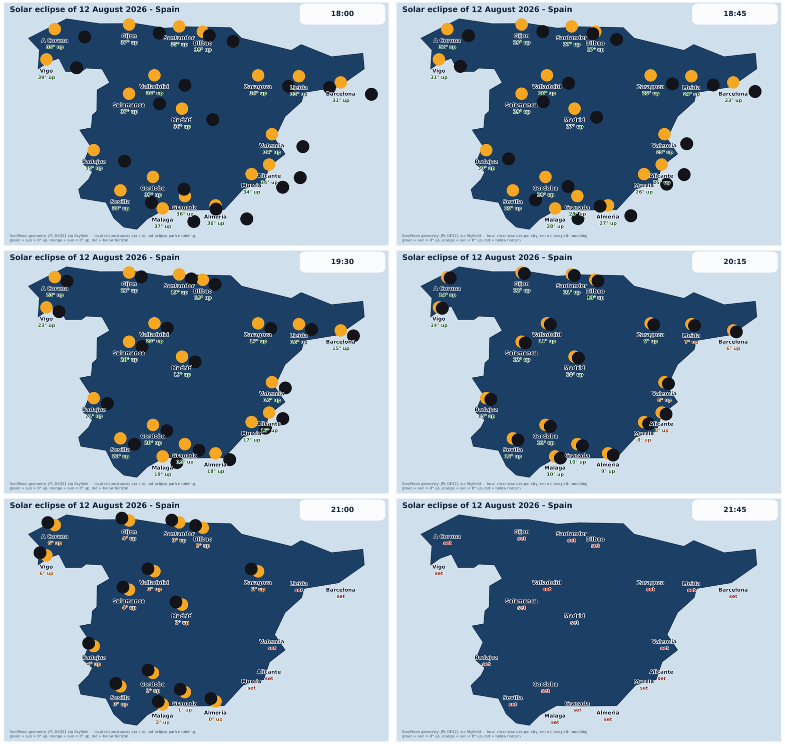
By 20:30 CEST several cities, Sevilla, Malaga, Almeria, Bilbao among them, are down to a thin crescent, while the cluster nearer the path of totality, Zaragoza, Lleida, Valladolid, Barcelona, has the Moon's disc fully covering the Sun's in this simplified geometry. The northwest coast, A Coruna and Vigo, drops out of the animation earliest: the Sun sets there while the eclipse is still in progress, and Madrid itself is down to about 8 degrees of altitude by the time the crescent is at its most dramatic.

What this is and isn't

This is a geometry sketch, not an eclipse calculator. A few specific simplifications worth naming:

No limb correction or refraction. Real eclipse predictions use Besselian elements and a measured lunar limb profile; this uses a spherical Moon and Sun and topocentric apparent positions straight from DE421, which is precise enough to get the shape and rough timing right but not to certify exact contact times or the precise edge of the path of totality.
The alt/az tangent-plane offset is an approximation. It's accurate for angular separations this small (well under a degree), but it's not the same construction professional eclipse cartography uses.
Cities are hidden below the horizon, not dimmed by twilight. The cutoff is sun_alt_deg > 0 exactly; real visibility fades out gradually before that, especially with any western horizon obstruction.
The altitude readout is the geometric horizon, not the visible one. A flat-horizon altitude of 7-8 degrees can still mean "blocked by a ridge to the west" depending on the specific terrain, especially anywhere mountainous; this data can't substitute for checking the actual horizon at a viewing spot.

For the actual times, path, and magnitude at a specific location, the usual authoritative sources, timeanddate.com or a national institute like the IAA-CSIC, are worth checking instead. This was built to answer a narrower question: whether a nice piece of eclipse graphic design travels well to a different country and a Python-only toolchain, and it does, in well under 350 lines, altitude readout and all.